Plotting
This notebook is part of the CaTabRa GitHub repository.
This short example demonstrates CaTabRa’s built-in plotting capabilities:
For a more thorough account on plotting in CaTabRa, please refer to Plots.
Familiarity with CaTabRa’s main data analysis workflow is assumed. A step-by-step introduction can be found in CaTabRa Workflow.
Create Plots in Python
When analyzing data and evaluating or explaining prediction models, CaTabRa automatically plots some of the results and saves the resulting figures as png, pdf or other files. For a more fine-grained control of plotting, there is also a Python API.
Let’s start with analyzing some data.
[2]:
# load dataset
from sklearn.datasets import load_breast_cancer
X, y = load_breast_cancer(as_frame=True, return_X_y=True)
[3]:
# add target labels to DataFrame
X['diagnosis'] = y
[4]:
# split into train- and test set by adding column with corresponding values
# the name of the column is arbitrary; CaTabRa tries to "guess" which samples belong to which set based on the column name and -values
X['train'] = X.index <= 0.8 * len(X)
[5]:
from catabra.analysis import analyze

analyze(
    X,
    classify='diagnosis',     # name of column containing classification target
    split='train',            # name of column containing information about the train-test split (optional)
    time=1,                   # time budget for hyperparameter tuning, in minutes (optional)
    out='plotting_example',
)
[CaTabRa] ### Analysis started at 2023-04-13 12:21:00.744873
[CaTabRa] Saving descriptive statistics completed
/mnt/c/Users/skaltenl/Documents/catabra_2023/develop/catabra/catabra/util/statistics.py:213: FutureWarning: The default value of numeric_only in DataFrame.corr is deprecated. In a future version, it will default to False. Select only valid columns or specify the value of numeric_only to silence this warning.
  return dict_stat, dict_non_num_stat, (df.corr() if df.shape[1] <= corr_threshold else None)
[CaTabRa] Using AutoML-backend auto-sklearn for binary_classification
[CaTabRa] Successfully loaded the following auto-sklearn add-on module(s): xgb
[CaTabRa] Using auto-sklearn 2.0.
/home/skaltenl/anaconda3/envs/test2/lib/python3.9/site-packages/autosklearn/experimental/selector.py:24: FutureWarning: iteritems is deprecated and will be removed in a future version. Use .items instead.
  for col, series in prediction.iteritems():
/home/skaltenl/anaconda3/envs/test2/lib/python3.9/site-packages/smac/intensification/parallel_scheduling.py:153: UserWarning: SuccessiveHalving is executed with 1 workers only. Consider to use pynisher to use all available workers.
  warnings.warn(
[CaTabRa] New ensemble fitted:
    ensemble_val_roc_auc: 0.986260
    n_constituent_models: 1
    total_elapsed_time: 00:05
[CaTabRa] New model #1 trained:
    val_roc_auc: 0.989845
    val_accuracy: 0.947368
    val_balanced_accuracy: 0.946356
    train_roc_auc: 1.000000
    type: gradient_boosting
    total_elapsed_time: 00:05
[CaTabRa] New ensemble fitted:
    ensemble_val_roc_auc: 0.986260
    n_constituent_models: 1
    total_elapsed_time: 00:08
[CaTabRa] New model #2 trained:
    val_roc_auc: 0.945430
    val_accuracy: 0.921053
    val_balanced_accuracy: 0.924134
    train_roc_auc: 1.000000
    type: gradient_boosting
    total_elapsed_time: 00:08
[CaTabRa] New ensemble fitted:
    ensemble_val_roc_auc: 0.986260
    n_constituent_models: 1
    total_elapsed_time: 00:10
[CaTabRa] New model #3 trained:
    val_roc_auc: 0.971416
    val_accuracy: 0.921053
    val_balanced_accuracy: 0.919952
    train_roc_auc: 0.993877
    type: gradient_boosting
    total_elapsed_time: 00:10
[CaTabRa] New ensemble fitted:
    ensemble_val_roc_auc: 0.987834
    n_constituent_models: 3
    total_elapsed_time: 00:13
[CaTabRa] New model #4 trained:
    val_roc_auc: 0.968250
    val_accuracy: 0.929825
    val_balanced_accuracy: 0.926523
    train_roc_auc: 0.995034
    type: gradient_boosting
    total_elapsed_time: 00:13
[CaTabRa] New ensemble fitted:
    ensemble_val_roc_auc: 0.996953
    n_constituent_models: 1
    total_elapsed_time: 00:16
[CaTabRa] New model #5 trained:
    val_roc_auc: 0.997073
    val_accuracy: 0.971491
    val_balanced_accuracy: 0.970072
    train_roc_auc: 0.999985
    type: mlp
    total_elapsed_time: 00:16
[CaTabRa] New ensemble fitted:
    ensemble_val_roc_auc: 0.996953
    n_constituent_models: 1
    total_elapsed_time: 00:18
[CaTabRa] New model #6 trained:
    val_roc_auc: 0.955048
    val_accuracy: 0.914474
    val_balanced_accuracy: 0.915233
    train_roc_auc: 0.986036
    type: gradient_boosting
    total_elapsed_time: 00:18
[CaTabRa] New ensemble fitted:
    ensemble_val_roc_auc: 0.996953
    n_constituent_models: 1
    total_elapsed_time: 00:21
[CaTabRa] New model #7 trained:
    val_roc_auc: 0.990054
    val_accuracy: 0.949561
    val_balanced_accuracy: 0.946535
    train_roc_auc: 1.000000
    type: gradient_boosting
    total_elapsed_time: 00:21
[CaTabRa] New ensemble fitted:
    ensemble_val_roc_auc: 0.997172
    n_constituent_models: 2
    total_elapsed_time: 00:23
[CaTabRa] New model #8 trained:
    val_roc_auc: 0.995579
    val_accuracy: 0.949561
    val_balanced_accuracy: 0.954898
    train_roc_auc: 0.996864
    type: mlp
    total_elapsed_time: 00:23
[CaTabRa] New ensemble fitted:
    ensemble_val_roc_auc: 0.997172
    n_constituent_models: 2
    total_elapsed_time: 00:26
[CaTabRa] New model #9 trained:
    val_roc_auc: 0.990352
    val_accuracy: 0.969298
    val_balanced_accuracy: 0.967384
    train_roc_auc: 0.999701
    type: mlp
    total_elapsed_time: 00:25
[CaTabRa] New ensemble fitted:
    ensemble_val_roc_auc: 0.997172
    n_constituent_models: 2
    total_elapsed_time: 00:28
[CaTabRa] New ensemble fitted:
    ensemble_val_roc_auc: 0.997172
    n_constituent_models: 2
    total_elapsed_time: 00:30
[CaTabRa] New model #10 trained:
    val_roc_auc: 0.988949
    val_accuracy: 0.936404
    val_balanced_accuracy: 0.937933
    train_roc_auc: 0.999955
    type: mlp
    total_elapsed_time: 00:30
[CaTabRa] New ensemble fitted:
    ensemble_val_roc_auc: 0.997172
    n_constituent_models: 2
    total_elapsed_time: 00:33
[CaTabRa] New model #11 trained:
    val_roc_auc: 0.992861
    val_accuracy: 0.964912
    val_balanced_accuracy: 0.962007
    train_roc_auc: 1.000000
    type: extra_trees
    total_elapsed_time: 00:32
[CaTabRa] New ensemble fitted:
    ensemble_val_roc_auc: 0.997172
    n_constituent_models: 2
    total_elapsed_time: 00:35
[CaTabRa] New model #12 trained:
    val_roc_auc: 0.991756
    val_accuracy: 0.953947
    val_balanced_accuracy: 0.951912
    train_roc_auc: 1.000000
    type: gradient_boosting
    total_elapsed_time: 00:35
[CaTabRa] New ensemble fitted:
    ensemble_val_roc_auc: 0.997172
    n_constituent_models: 2
    total_elapsed_time: 00:37
[CaTabRa] New ensemble fitted:
    ensemble_val_roc_auc: 0.997172
    n_constituent_models: 2
    total_elapsed_time: 00:40
[CaTabRa] New model #13 trained:
    val_roc_auc: 0.995639
    val_accuracy: 0.964912
    val_balanced_accuracy: 0.961171
    train_roc_auc: 0.999044
    type: mlp
    total_elapsed_time: 00:40
[CaTabRa] New ensemble fitted:
    ensemble_val_roc_auc: 0.997172
    n_constituent_models: 2
    total_elapsed_time: 00:43
[CaTabRa] New model #14 trained:
    val_roc_auc: 0.993429
    val_accuracy: 0.967105
    val_balanced_accuracy: 0.964695
    train_roc_auc: 0.999836
    type: extra_trees
    total_elapsed_time: 00:42
[CaTabRa] New ensemble fitted:
    ensemble_val_roc_auc: 0.997172
    n_constituent_models: 2
    total_elapsed_time: 00:47
[CaTabRa] New model #15 trained:
    val_roc_auc: 0.958393
    val_accuracy: 0.888158
    val_balanced_accuracy: 0.889665
    train_roc_auc: 0.973305
    type: gradient_boosting
    total_elapsed_time: 00:49
[CaTabRa] New model #16 trained:
    val_roc_auc: 0.989934
    val_accuracy: 0.947368
    val_balanced_accuracy: 0.944683
    train_roc_auc: 0.997961
    type: gradient_boosting
    total_elapsed_time: 00:51
/home/skaltenl/anaconda3/envs/test2/lib/python3.9/site-packages/sklearn/preprocessing/_data.py:3237: RuntimeWarning: divide by zero encountered in log
  loglike = -n_samples / 2 * np.log(x_trans.var())
/home/skaltenl/anaconda3/envs/test2/lib/python3.9/site-packages/sklearn/neural_network/_multilayer_perceptron.py:614: ConvergenceWarning: Stochastic Optimizer: Maximum iterations (32) reached and the optimization hasn't converged yet.
  warnings.warn(
/home/skaltenl/anaconda3/envs/test2/lib/python3.9/site-packages/sklearn/neural_network/_multilayer_perceptron.py:614: ConvergenceWarning: Stochastic Optimizer: Maximum iterations (32) reached and the optimization hasn't converged yet.
  warnings.warn(
[CaTabRa] Final training statistics:
    n_models_trained: 16
    ensemble_val_roc_auc: 0.9971724412584628
[CaTabRa] Creating shap explainer
[CaTabRa] Initialized out-of-distribution detector of type BinsDetector
[CaTabRa] Fitting out-of-distribution detector...
[CaTabRa] Out-of-distribution detector fitted.
[CaTabRa] ### Analysis finished at 2023-04-13 12:21:59.989624
[CaTabRa] ### Elapsed time: 0 days 00:00:59.244751
[CaTabRa] ### Output saved in /mnt/c/Users/skaltenl/Documents/catabra_2023/develop/catabra/examples/plotting_example
[CaTabRa] ### Evaluation started at 2023-04-13 12:22:00.008499
[CaTabRa] Saving descriptive statistics completed
[CaTabRa] Predicting out-of-distribution samples.
The default value of numeric_only in DataFrame.corr is deprecated. In a future version, it will default to False. Select only valid columns or specify the value of numeric_only to silence this warning.
[CaTabRa] Saving descriptive statistics completed
[CaTabRa] Predicting out-of-distribution samples.
[CaTabRa] Evaluation results for train:
    roc_auc: 0.9990442054958184
    accuracy @ 0.5: 0.9824561403508771
    balanced_accuracy @ 0.5: 0.9818399044205496
The default value of numeric_only in DataFrame.corr is deprecated. In a future version, it will default to False. Select only valid columns or specify the value of numeric_only to silence this warning.
[CaTabRa] Evaluation results for not_train:
    roc_auc: 0.9995579133510168
    accuracy @ 0.5: 0.9734513274336283
    balanced_accuracy @ 0.5: 0.9827586206896552
[CaTabRa] ### Evaluation finished at 2023-04-13 12:22:02.811294
[CaTabRa] ### Elapsed time: 0 days 00:00:02.802795
[CaTabRa] ### Output saved in /mnt/c/Users/skaltenl/Documents/catabra_2023/develop/catabra/examples/plotting_example/eval
Recall from CaTabRa Workflow that by specifying a train-test split the final classifier is automatically evaluated after training. The resulting figures are saved in eval/train/static_plots/ and eval/not_train/static_plots. But we can create (and modify) them directly in Python, too.
[6]:
from catabra.util.io import CaTabRaLoader

loader = CaTabRaLoader('plotting_example')
Create performance plots for the test set:
[7]:
from catabra.evaluation import plot_results

figures = plot_results(
    loader.path / 'eval/not_train/predictions.xlsx',    # table with predictions for all samples
    loader.path / 'eval/not_train/metrics.xlsx',        # table with performance metrics
    loader.get_encoder()                                # data encoder
)
The result is a dict mapping keys to `matplotlib.pyplot.Figure <https://matplotlib.org/stable/api/figure_api.html#matplotlib.figure.Figure>`__ instances. The keys correspond precisely to the names of the figure-files in eval/not_train/static_plots/.
[8]:
figures.keys()
[8]:
dict_keys(['roc_curve', 'pr_curve', 'threshold', 'confusion_matrix', 'calibration'])
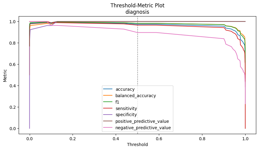
[9]:
figures['threshold']
[9]:
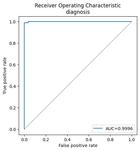
[10]:
figures['roc_curve']
[10]:
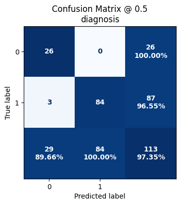
[11]:
figures['confusion_matrix']
[11]:
There are similar ways to plot training history and feature importance. Check out Plots for details.
Create Interactive Plots with plotly
So far, all plots were created with the default Matplotlib backend. CaTabRa can be instructed to produce interactive plots using the plotly backend with only a few lines of code.
Since plotly is not installed by default, we have to install it manually (using either pip or conda):
[12]:
!pip install plotly==5.7.0
WARNING: Ignoring invalid distribution -ytest (/home/skaltenl/anaconda3/envs/test2/lib/python3.9/site-packages)
WARNING: Ignoring invalid distribution -lotly (/home/skaltenl/anaconda3/envs/test2/lib/python3.9/site-packages)
WARNING: Ignoring invalid distribution -ytest (/home/skaltenl/anaconda3/envs/test2/lib/python3.9/site-packages)
WARNING: Ignoring invalid distribution -lotly (/home/skaltenl/anaconda3/envs/test2/lib/python3.9/site-packages)
Requirement already satisfied: plotly==5.7.0 in /home/skaltenl/anaconda3/envs/test2/lib/python3.9/site-packages (5.7.0)
Requirement already satisfied: six in /home/skaltenl/anaconda3/envs/test2/lib/python3.9/site-packages (from plotly==5.7.0) (1.16.0)
Requirement already satisfied: tenacity>=6.2.0 in /home/skaltenl/anaconda3/envs/test2/lib/python3.9/site-packages (from plotly==5.7.0) (8.2.2)
WARNING: Ignoring invalid distribution -ytest (/home/skaltenl/anaconda3/envs/test2/lib/python3.9/site-packages)
WARNING: Ignoring invalid distribution -lotly (/home/skaltenl/anaconda3/envs/test2/lib/python3.9/site-packages)
WARNING: Ignoring invalid distribution -ytest (/home/skaltenl/anaconda3/envs/test2/lib/python3.9/site-packages)
WARNING: Ignoring invalid distribution -lotly (/home/skaltenl/anaconda3/envs/test2/lib/python3.9/site-packages)
WARNING: Ignoring invalid distribution -ytest (/home/skaltenl/anaconda3/envs/test2/lib/python3.9/site-packages)
WARNING: Ignoring invalid distribution -lotly (/home/skaltenl/anaconda3/envs/test2/lib/python3.9/site-packages)
WARNING: Ignoring invalid distribution -ytest (/home/skaltenl/anaconda3/envs/test2/lib/python3.9/site-packages)
WARNING: Ignoring invalid distribution -lotly (/home/skaltenl/anaconda3/envs/test2/lib/python3.9/site-packages)
For automatically creating interactive plots during all stages of CaTabRa’s data analysis workflow we can update the config dict passed to the initial call to analyze(). The config dict can be updated by either passing a dict or the path to a JSON file containing such a dict; the latter is especially useful on the command line.
NOTE For more information about the possible config parameters and their meaning, please refer to Configuration.
[13]:
analyze(
    X,
    classify='diagnosis',     # name of column containing classification target
    split='train',            # name of column containing information about the train-test split (optional)
    time=1,                   # time budget for hyperparameter tuning, in minutes (optional)
    out='plotting_example_interactive',
    config={
        'static_plots': True,         # whether to create static plots; True by default
        'interactive_plots': True     # whether to create interactive plots; False by default
    }
)
[CaTabRa] ### Analysis started at 2023-04-13 12:22:05.167578
[CaTabRa] Saving descriptive statistics completed
[CaTabRa] Using AutoML-backend auto-sklearn for binary_classification
[CaTabRa] Successfully loaded the following auto-sklearn add-on module(s): xgb
[CaTabRa] Using auto-sklearn 2.0.
The default value of numeric_only in DataFrame.corr is deprecated. In a future version, it will default to False. Select only valid columns or specify the value of numeric_only to silence this warning.
iteritems is deprecated and will be removed in a future version. Use .items instead.
SuccessiveHalving is executed with 1 workers only. Consider to use pynisher to use all available workers.
[CaTabRa] New ensemble fitted:
    ensemble_val_roc_auc: 0.986260
    n_constituent_models: 1
    total_elapsed_time: 00:03
[CaTabRa] New model #1 trained:
    val_roc_auc: 0.989845
    val_accuracy: 0.947368
    val_balanced_accuracy: 0.946356
    train_roc_auc: 1.000000
    type: gradient_boosting
    total_elapsed_time: 00:03
[CaTabRa] New ensemble fitted:
    ensemble_val_roc_auc: 0.986260
    n_constituent_models: 1
    total_elapsed_time: 00:05
[CaTabRa] New model #2 trained:
    val_roc_auc: 0.945430
    val_accuracy: 0.921053
    val_balanced_accuracy: 0.924134
    train_roc_auc: 1.000000
    type: gradient_boosting
    total_elapsed_time: 00:05
[CaTabRa] New ensemble fitted:
    ensemble_val_roc_auc: 0.986260
    n_constituent_models: 1
    total_elapsed_time: 00:08
[CaTabRa] New model #3 trained:
    val_roc_auc: 0.971416
    val_accuracy: 0.921053
    val_balanced_accuracy: 0.919952
    train_roc_auc: 0.993877
    type: gradient_boosting
    total_elapsed_time: 00:08
[CaTabRa] New ensemble fitted:
    ensemble_val_roc_auc: 0.987834
    n_constituent_models: 3
    total_elapsed_time: 00:10
[CaTabRa] New model #4 trained:
    val_roc_auc: 0.968250
    val_accuracy: 0.929825
    val_balanced_accuracy: 0.926523
    train_roc_auc: 0.995034
    type: gradient_boosting
    total_elapsed_time: 00:10
[CaTabRa] New ensemble fitted:
    ensemble_val_roc_auc: 0.996953
    n_constituent_models: 1
    total_elapsed_time: 00:14
[CaTabRa] New model #5 trained:
    val_roc_auc: 0.997073
    val_accuracy: 0.971491
    val_balanced_accuracy: 0.970072
    train_roc_auc: 0.999985
    type: mlp
    total_elapsed_time: 00:13
[CaTabRa] New ensemble fitted:
    ensemble_val_roc_auc: 0.996953
    n_constituent_models: 1
    total_elapsed_time: 00:16
[CaTabRa] New model #6 trained:
    val_roc_auc: 0.955048
    val_accuracy: 0.914474
    val_balanced_accuracy: 0.915233
    train_roc_auc: 0.986036
    type: gradient_boosting
    total_elapsed_time: 00:15
[CaTabRa] New ensemble fitted:
    ensemble_val_roc_auc: 0.996953
    n_constituent_models: 1
    total_elapsed_time: 00:18
[CaTabRa] New model #7 trained:
    val_roc_auc: 0.990054
    val_accuracy: 0.949561
    val_balanced_accuracy: 0.946535
    train_roc_auc: 1.000000
    type: gradient_boosting
    total_elapsed_time: 00:18
[CaTabRa] New ensemble fitted:
    ensemble_val_roc_auc: 0.997172
    n_constituent_models: 2
    total_elapsed_time: 00:20
[CaTabRa] New model #8 trained:
    val_roc_auc: 0.995579
    val_accuracy: 0.949561
    val_balanced_accuracy: 0.954898
    train_roc_auc: 0.996864
    type: mlp
    total_elapsed_time: 00:20
[CaTabRa] New ensemble fitted:
    ensemble_val_roc_auc: 0.997172
    n_constituent_models: 2
    total_elapsed_time: 00:23
[CaTabRa] New model #9 trained:
    val_roc_auc: 0.990352
    val_accuracy: 0.969298
    val_balanced_accuracy: 0.967384
    train_roc_auc: 0.999701
    type: mlp
    total_elapsed_time: 00:23
[CaTabRa] New ensemble fitted:
    ensemble_val_roc_auc: 0.997172
    n_constituent_models: 2
    total_elapsed_time: 00:25
[CaTabRa] New ensemble fitted:
    ensemble_val_roc_auc: 0.997172
    n_constituent_models: 2
    total_elapsed_time: 00:28
[CaTabRa] New model #10 trained:
    val_roc_auc: 0.988949
    val_accuracy: 0.936404
    val_balanced_accuracy: 0.937933
    train_roc_auc: 0.999955
    type: mlp
    total_elapsed_time: 00:27
[CaTabRa] New ensemble fitted:
    ensemble_val_roc_auc: 0.997172
    n_constituent_models: 2
    total_elapsed_time: 00:30
[CaTabRa] New model #11 trained:
    val_roc_auc: 0.992861
    val_accuracy: 0.964912
    val_balanced_accuracy: 0.962007
    train_roc_auc: 1.000000
    type: extra_trees
    total_elapsed_time: 00:30
[CaTabRa] New ensemble fitted:
    ensemble_val_roc_auc: 0.997172
    n_constituent_models: 2
    total_elapsed_time: 00:32
[CaTabRa] New model #12 trained:
    val_roc_auc: 0.991756
    val_accuracy: 0.953947
    val_balanced_accuracy: 0.951912
    train_roc_auc: 1.000000
    type: gradient_boosting
    total_elapsed_time: 00:32
[CaTabRa] New ensemble fitted:
    ensemble_val_roc_auc: 0.997172
    n_constituent_models: 2
    total_elapsed_time: 00:35
[CaTabRa] New ensemble fitted:
    ensemble_val_roc_auc: 0.997172
    n_constituent_models: 2
    total_elapsed_time: 00:38
[CaTabRa] New model #13 trained:
    val_roc_auc: 0.995639
    val_accuracy: 0.964912
    val_balanced_accuracy: 0.961171
    train_roc_auc: 0.999044
    type: mlp
    total_elapsed_time: 00:37
[CaTabRa] New ensemble fitted:
    ensemble_val_roc_auc: 0.997172
    n_constituent_models: 2
    total_elapsed_time: 00:40
[CaTabRa] New model #14 trained:
    val_roc_auc: 0.993429
    val_accuracy: 0.967105
    val_balanced_accuracy: 0.964695
    train_roc_auc: 0.999836
    type: extra_trees
    total_elapsed_time: 00:40
[CaTabRa] New ensemble fitted:
    ensemble_val_roc_auc: 0.997172
    n_constituent_models: 2
    total_elapsed_time: 00:44
[CaTabRa] New model #15 trained:
    val_roc_auc: 0.958393
    val_accuracy: 0.888158
    val_balanced_accuracy: 0.889665
    train_roc_auc: 0.973305
    type: gradient_boosting
    total_elapsed_time: 00:46
[CaTabRa] New model #16 trained:
    val_roc_auc: 0.989934
    val_accuracy: 0.947368
    val_balanced_accuracy: 0.944683
    train_roc_auc: 0.997961
    type: gradient_boosting
    total_elapsed_time: 00:48
divide by zero encountered in log
Stochastic Optimizer: Maximum iterations (32) reached and the optimization hasn't converged yet.
Stochastic Optimizer: Maximum iterations (32) reached and the optimization hasn't converged yet.
[CaTabRa] Final training statistics:
    n_models_trained: 16
    ensemble_val_roc_auc: 0.9971724412584628
[CaTabRa] Creating shap explainer
[CaTabRa] Initialized out-of-distribution detector of type BinsDetector
[CaTabRa] Fitting out-of-distribution detector...
[CaTabRa] Out-of-distribution detector fitted.
[CaTabRa] ### Analysis finished at 2023-04-13 12:23:02.650250
[CaTabRa] ### Elapsed time: 0 days 00:00:57.482672
[CaTabRa] ### Output saved in /mnt/c/Users/skaltenl/Documents/catabra_2023/develop/catabra/examples/plotting_example_interactive
[CaTabRa] ### Evaluation started at 2023-04-13 12:23:02.652969
[CaTabRa] Saving descriptive statistics completed
[CaTabRa] Predicting out-of-distribution samples.
/mnt/c/Users/skaltenl/Documents/catabra_2023/develop/catabra/catabra/util/statistics.py:213: FutureWarning:

The default value of numeric_only in DataFrame.corr is deprecated. In a future version, it will default to False. Select only valid columns or specify the value of numeric_only to silence this warning.
[CaTabRa] Saving descriptive statistics completed
[CaTabRa] Predicting out-of-distribution samples.
[CaTabRa] Evaluation results for train:
    roc_auc: 0.9990442054958184
    accuracy @ 0.5: 0.9824561403508771
    balanced_accuracy @ 0.5: 0.9818399044205496
/mnt/c/Users/skaltenl/Documents/catabra_2023/develop/catabra/catabra/util/statistics.py:213: FutureWarning:

The default value of numeric_only in DataFrame.corr is deprecated. In a future version, it will default to False. Select only valid columns or specify the value of numeric_only to silence this warning.
[CaTabRa] Evaluation results for not_train:
    roc_auc: 0.9995579133510168
    accuracy @ 0.5: 0.9734513274336283
    balanced_accuracy @ 0.5: 0.9827586206896552
[CaTabRa] ### Evaluation finished at 2023-04-13 12:23:05.557959
[CaTabRa] ### Elapsed time: 0 days 00:00:02.904990
[CaTabRa] ### Output saved in /mnt/c/Users/skaltenl/Documents/catabra_2023/develop/catabra/examples/plotting_example_interactive/eval
Looking at eval/train/ and eval/not_train/ in the newly created plotting_example_interactive you will now find folders static_plots (as before), but also interactive_plots. The latter contain HTML files with plotly-generated interactive plots that can be viewed in any modern browser.
In addition, it is also possible to create interactive plots directly in Python. Continuing the example from above, all we have to do is pass interactive=True to function plot_results():
[14]:
figures = plot_results(
    loader.path / 'eval/not_train/predictions.xlsx',    # table with predictions for all samples
    loader.path / 'eval/not_train/metrics.xlsx',        # table with performance metrics
    loader.get_encoder(),                               # data encoder
    interactive=True
)
The output is again a dict mapping keys to figures, but this time the figures are plotly figure instances:
[15]:
figures['threshold']
[16]:
figures['roc_curve']
[17]:
figures['confusion_matrix']
NOTE Every static Matplotlib figure that can be created in CaTabRa’s main data analysis workflow has an interactive plotly analogue, and vice versa. This includes training history plots, model performance plots and feature importance plots.